Frequency filtering in SkiaSharp
Previously, I wrote about performing convolution in SkiaSharp. I used the CreateMatrixConvolution method from the SKImageFilter class to convolve kernels with the source image. This method allows you to specify kernels of arbitrary size, allows you to specify how the edge pixels in the image are handled, and is lightning fast. I was particularly impressed with the execution speed of the method when considering the resolution of images these days, and the amount of processing that’s performed when convolving an image with a kernel, particularly for larger kernels.
In this blog post I’ll discuss implementing frequency filtering in SkiaSharp.
Frequency filtering
As any computer science undergrad can tell you, a Fourier transform takes a signal from the time domain and transforms it into the frequency domain. What this means is it takes a signal and decomposes it into its constituent frequencies. The world of signal processing is full of applications for the Fourier transform, with one of the standard applications being musical instrument tuners, which compare the frequency of sound input to the known frequencies of specific notes. Fourier transforms can be performed using analog electronics, digital electronics, and even at the speed of light using optics. For more information about the Fourier transform, see Fourier transform.
Another standard application of the Fourier transform is to perform frequency filtering. A signal can be transformed to the frequency domain, where specific frequencies, or frequency ranges, can be removed. This enables a class of filters to be implemented, known as pass through filters: specifically high-pass, low-pass, and band-pass filters. In terms of image processing, a low-pass filter attentuates high frequencies and retains low frequencies unchanged, with the result being similar to that of a smoothing filter. A high-pass filter attenuates low frequencies, and retains high frequencies unchanged, with the result being similar to that of edge detection. A band-pass filter attentuates very low and very high frequencies, but retains a middle band of frequencies, and is often used to enhance edges while reducing noise.
In terms of image processing, the Fourier transform transforms an image from the spatial domain to the frequency domain, where frequency filtering can then be performed. The process of performing frequency filtering on an image is:
- Fourier transform the image.
- Filter the image frequencies in the frequency domain.
- Inverse Fourier transform the frequency data back into the spatial domain.
In reality, the process of Fourier transforming an image is more complex than I’ve suggested. The frequency data that results from a Fourier transform is expressed as a complex number (a number that has a real, and imaginary component), whose magnitude represents the amount of that frequency present in the original signal, with the phase offset being the basic sinusoid in that frequency. For more information about complex numbers, see Complex number.
In addition, as well as handling complex numbers, there are other issues to be dealt with when Fourier transforming an image. Firstly, computing a Fourier transform is too slow to be practical, because it has a complexity of O(N2). However, this issue can be overcome by implementing a Fast Fourier Transform (FFT), which has a complexity of O(N log N). For more information about this algorithm, see Fast Fourier transform. Secondly, Fourier transforms only operate on image dimensions that are a power of 2 (512x512, 1024x1024 etc.). While there are techniques to allow arbitratily dimensioned images to be Fourier transformed, they are beyond the scope of this post. Therefore, any images processed by the algorithm must first be resized. Thirdly, which image data do you Fourier transform? RGBA channels? An alternative colour model such as YCbCr or YUV? The answer is to Fourier transform a greyscale representation of the image, as it’s the intensity data that carries more information than colour channels.
Implementing frequency filtering
I’ve made the following assumptions for my implementation:
- The input image for the Fourier transform will be a 32-bit image, with RGBA channels.
- The input image dimensions must be a power of 2. This is due to the FFT algorithm (Radix-2 FFT) being used.
- The input image will first be converted to a greyscale representation.
- The greyscale representation will then be converted to a complex number representation.
- The complex number data will undergo a 2D FFT.
- Filtering will then be performed in the frequency domain.
- The filtered complex data will be inverse FFT’d.
- The filtered complex data will be converted back from complex numbers to pixel data for display.
- The output image will be in greyscale, but still stored as an RGBA image.
It takes more code to implement a 2D FFT than can be covered here, particularly as there are complexities I haven’t discussed. Rather than show every last bit of code, I’ll just state that there’s a Complex type that represents a complex number, and a ComplexImage type that represents an image as a 2D array of complex numbers. The full source code can be found on GitHub.
The following code shows a high level overview of how frequency filtering is implemented:
public static unsafe SKPixmap FrequencyFilter(this SKBitmap bitmap, int min, int max)
{
    ComplexImage complexImage = bitmap.ToComplexImage();

    complexImage.FastFourierTransform();
    FrequencyFilter filter = new FrequencyFilter(new FrequencyRange(min, max));
    filter.Apply(complexImage);
    complexImage.ReverseFastFourierTransform();

    SKPixmap pixmap = complexImage.ToSKPixmap(bitmap);
    return pixmap;
}
This method converts the image to a ComplexImage object, which then undergoes a 2D FFT. A FrequencyFilter object is then created, based on the values of Slider elements on the UI. The filter is applied to the ComplexImage object, and then inverse FFT’d before being converted back to pixel data.
Note: There are plenty of opportunities to optimise my FFT implementation, as it focuses on clarity rather than performance. In particular, a 2D FFT naturally lends itself to parallelisation.
A Fourier transform produces a complex number valued output image that can be displayed as two images, for the real and imaginary coefficients, or as their magnitude and phase. In image processing, it’s usually the magnitude of the Fourier transform that’s displayed, as it contains most of the information about the geometric structure of the source image. However, to inverse transform the data after procesing in the frequency domain, both the magnitude and phase of the Fourier data is required and so must be preserved.
It’s possible to view the Fourier transformed image, known as a frequency spectra, by commenting out a couple of lines in the FrequencyFilter method. I mentioned earlier that there are additional complexities when implementing a FFT, and one of them is that the dynamic range of Fourier coefficients is too large to be displayed in an image, and the resulting image would appear all black. However, if a logarithmic transformation is applied to the coefficients, which the source does, the frequency spectra can be displayed:
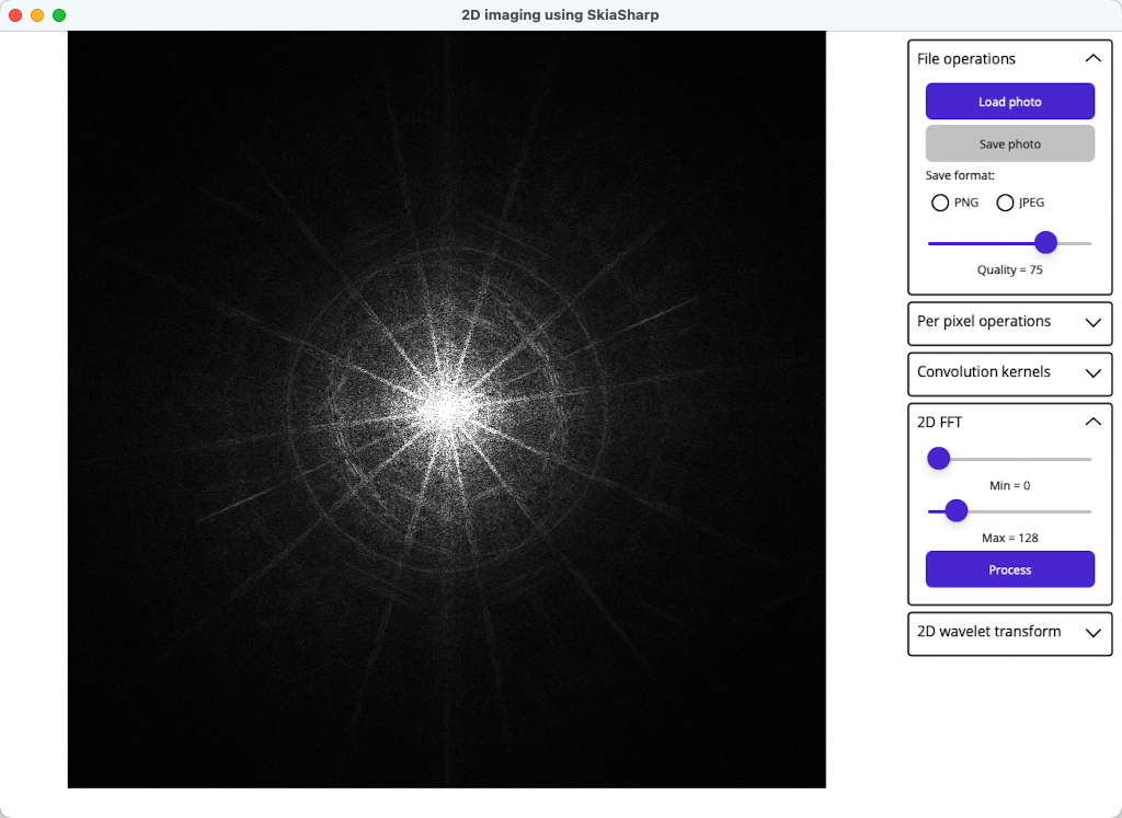
The image is shifted so that frequency (0,0) is displayed at the center of the image. The further away from the center a point in the image is, the higher is its corresponding frequency. Therefore, the blob at the center of the image tells us that the image largely consists of lower frequencies. The spectra also tells us that there are are lines in many different directions in the image, which are a result of the spokes on the big wheel.
Frequency filtering is performed by the Apply method in the FrequencyFilter class:
public void Apply(ComplexImage complexImage)
{
    if (!complexImage.IsFourierTransformed)
    {
        throw new ArgumentException("The source complex image should be Fourier transformed.");
    }

    int width = complexImage.Width;
    int height = complexImage.Height;
    int halfWidth = width >> 1;
    int halfHeight = height >> 1;
    int min = _frequencyRange.Min;
    int max = _frequencyRange.Max;

    Complex[,] data = complexImage.Data;
    for (int i = 0; i < height; i++)
    {
        int y = i - halfHeight;
        for (int j = 0; j < width; j++)
        {
            int x = j - halfWidth;
            int d = (int)Math.Sqrt(x * x + y * y);

            if ((d > max) || (d < min))
            {
                data[i, j].Re = 0;
                data[i, j].Im = 0;
            }
        }
    }
}
This method iterates over the complex image data, and zeroes the real and imaginery values that lie outside the frequency range specified by the min and max values. Conversely, frequency data within the min and max values are passed through. Therefore, this method implements a band-pass filter that can be configured to operate at any frequency range.
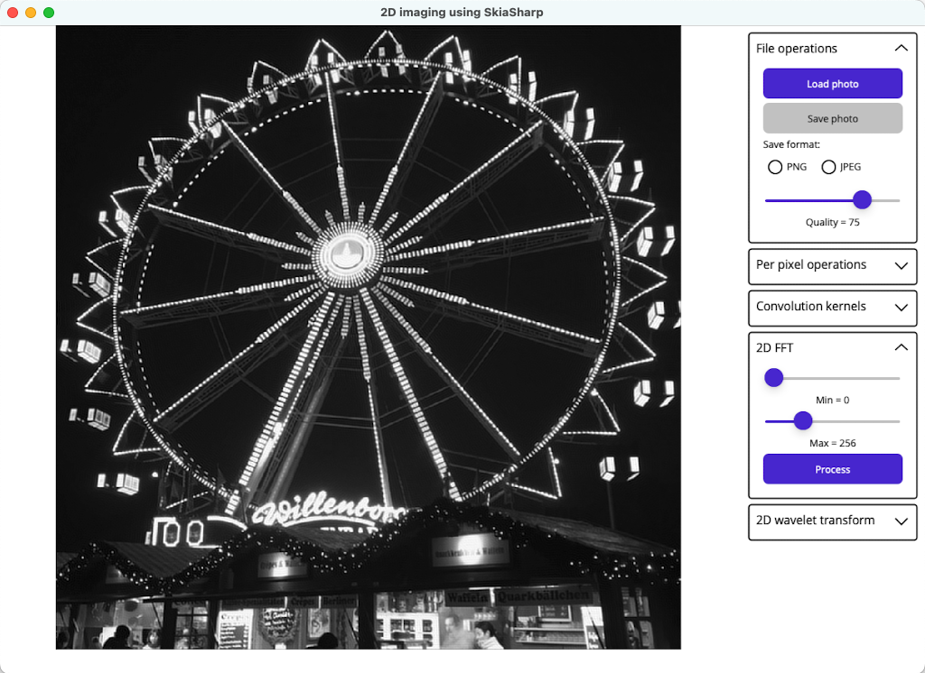
Because the earlier spectra showed that the image largely consists of low frequency data, a frequency filter with a min value of 0 and a max value of 256 results in a greyscale representation of the original source image that’s largely perfect:
However, a frequency filter with a min value of 10 and a max value of 128 yields the following image:
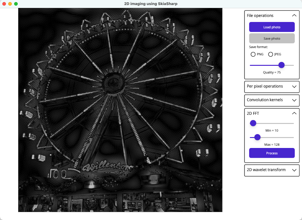
In this image, because some of the low frequency data has been removed, only sharp changes in intensity values are being preserved, with the resulting image beginning to look as if it’s been edge detected. Similarly, a frequency filter with a min value of 20 and a max value of 128 furthers this effect:
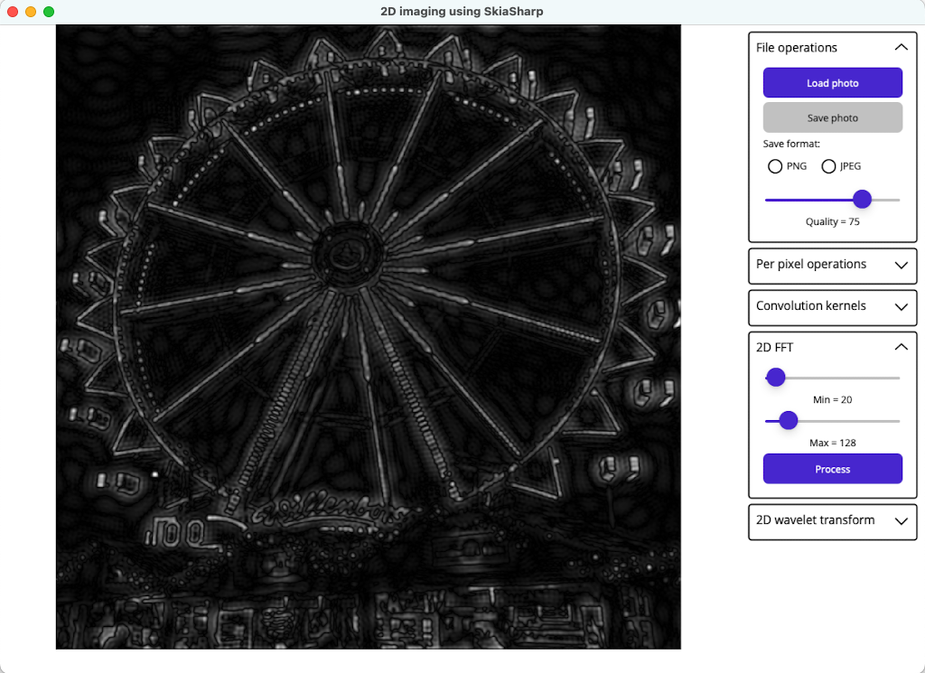
Again, the output is now looking even more like the output of an edge detector.
Consumer imaging apps don’t typically contain operations that Fourier transform image data. However, it’s a mainstay of scientific imaging. One of the main uses of frequency filtering in image processing is to remove noise. If the frequency range of the noise can be identified, which it often can be, that frequency range can be removed resulting in a denoised image. Another real world application of the Fourier transform in imaging is producing images of steel rebar quality inside concrete. In this case, transducer data can be deconvolved in the frequency domain with the point spread function of the transducer, to yield images of steel rebar quality inside concrete, from which any potential deterioration can be identified.